
Tutorial - Working with Tabular Data
This tutorial explores how MATLAB and Kornucopia handle tabular data. The example also discusses several important concepts regarding Kornucopia's Units features.
Contents
- Overview
- Set-up
- Initial viewing of the data
- Displaying some pictures of how the variables display in MATLAB
- Convert FEA_t to a k_units data type
- Display picture of 5 possible ways to view k_units variable in MATLAB
- Viewing the Kornucopia Units Library
- Convert exper_t to k_units data type
- Define unit of 'g' and re-attempt converting exper_t to k_units
- Compare the FEA and Experimental Data
- Comparing displacements by integrating accelerations
- Convert the FEA and Exper variables to a common Units Pref
- Shift time of Experiment and replot
- Shift time of Experiment using units and replot
- Convert to US Customary units and make time in msec, then replot
- Demonstration of computing a derivative
- Options to save figure windows
- End of example & optional clean-up
Overview
%{
The tutorial covers the following:
 o Utilizing Units with all calculations.
    - This will include working with US Customary units and metric
      units, as well as a mix of these units.
    - Also demonstrated are several supported approaches to associate
      units with data and to work with variables.
 o Some similarities and differences between MATLAB table data type &
   Kornucopia k_units data type are also presented.

Tips:
 o Consider running the example "By Section". It will help you walk
   through the example and its results.
%}
Set-up
%{
This section makes a few initial settings for the example.

Additional Details:
The settings below include:
 o Popup asking to clean MATLAB session before start of example.
 o Saving your current settings for all ADV settings, Units
   Preference, and MATLAB format. These will be reset to their
   respective values at the end of the example.
 o Define a handy "adv" variable so that we can later use it to
   quickly access any Kornucopia function's ADV options with ease.
 o Setting a specific Units Preference for the beginning of the
   example.
 o Loading two variables from a single MAT file into the session.
   The variables being loaded are MATLAB tables.
 o A warning message that some intentional errors will be created in
   this example.
 o The last 2 lines in this section suppress two MATLAB editor
   warnings:
    - "%#ok<*NOPTS>" suppresses warning of "no ;" at end of commands.
      Occasionally we will be omitting the ";" at the end of commands
      to allow their values to echo to the command window.
    - "%#ok<*NASGU>" suppresses warning that variable is not used. We
      occasionally create such a variable when showing variables in
      different units.

*** Tip ***
In some of the sections below, you will be told to manually enter some
commands into the MATLAB command window. The commands to use are
generally shown in the comment section. You can simply highlight the
commands and hit "F9" (no quotes) to have the commands executed into
the MATLAB command window.
%}

k_cleanup({'BEFORE starting the example:'; ' '});
origSettings = k_exampleSetup();
adv = k_adv();

k_unitsPreferenceActivate('mm_N_ms');

% Load two variables that each hold a MATLAB table
k_examplesOpen('lensImpactData_T', 'loadMat', 'on')

msgTxt = {'*** PLEASE READ ***'; ...
          'There will be one or more places in this' ; ...
          'example that INTENTIONALLY create an'; ...
          'error to show you how Kornucopia handles'; ...
          'errors. Please read the messages produced'; ...
          'and their related comments in the m-file.'};
warndlg(msgTxt, 'PLEASE READ');

%#ok<*NOPTS>
%#ok<*NASGU>
Units Preference now activated: 'mm_N_ms'

Kornucopia Examples MAT file, 'lensImpactData_T' is loaded into MATLAB session.
Initial viewing of the data
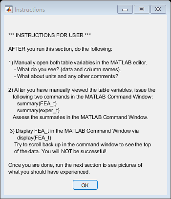
%{
Two MATLAB tables were loaded into the session:
 o FEA_t
 o exper_t

%}

txt = {
    '*** INSTRUCTIONS FOR USER ***'
    ' '
    'AFTER you run this section, do the following:'
    ' '
    '1) Manually open both table variables in the MATLAB editor. '
    '    - What do you see? (data and column names). '
    '    - What about units and any other comments? '
    ' '
    '2) After you have manually viewed the table variables, issue the '
    '   following two commands in the MATLAB Command Window: '
    '      summary(FEA_t)'
    '      summary(exper_t)'
    '   Assess the summaries in the MATLAB Command Window. '
    ' '
    ' 3) Display FEA_t in the MATLAB Command Window via '
    '      display(FEA_t) '
    '    Try to scroll back up in the command window to see the top '
    '    of the data. You will NOT be successful! '
    ' '
    'Once you are done, run the next section to see pictures of '
    'what you should have experienced. '
    };

msgbox(txt, 'Instructions');
Displaying some pictures of how the variables display in MATLAB
figH = figure('position', k_figZoom(1.75));
titles = {'Three Views FEA_t', 'Three Views exper_t'};
tabStuff = k_figTabsCreate(titles, figH);

dataDir = k_examplesDir('data');

currentTabH = tabStuff.TabsH(1);
imageName = 'threeViews_FEA_t.png';
fullImageName = fullfile(dataDir, 'media', imageName);
k_picDisplay(fullImageName, 'center', ...
    'parent', currentTabH);
k_figTabsDisplay(currentTabH);

currentTabH = tabStuff.TabsH(2);
imageName = 'threeViews_exper_t.png';
fullImageName = fullfile(dataDir, 'media', imageName);
k_picDisplay(fullImageName, 'center', ...
    'parent', currentTabH);
k_figTabsDisplay(currentTabH);

txt = 'Two tabs were created in the figure that just appeared. Explore them both';
msgbox(txt);

Convert FEA_t to a k_units data type
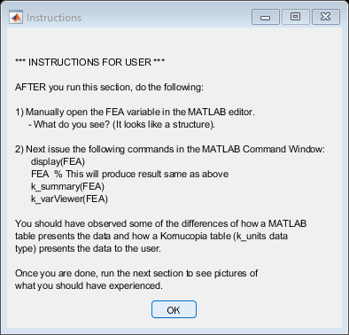
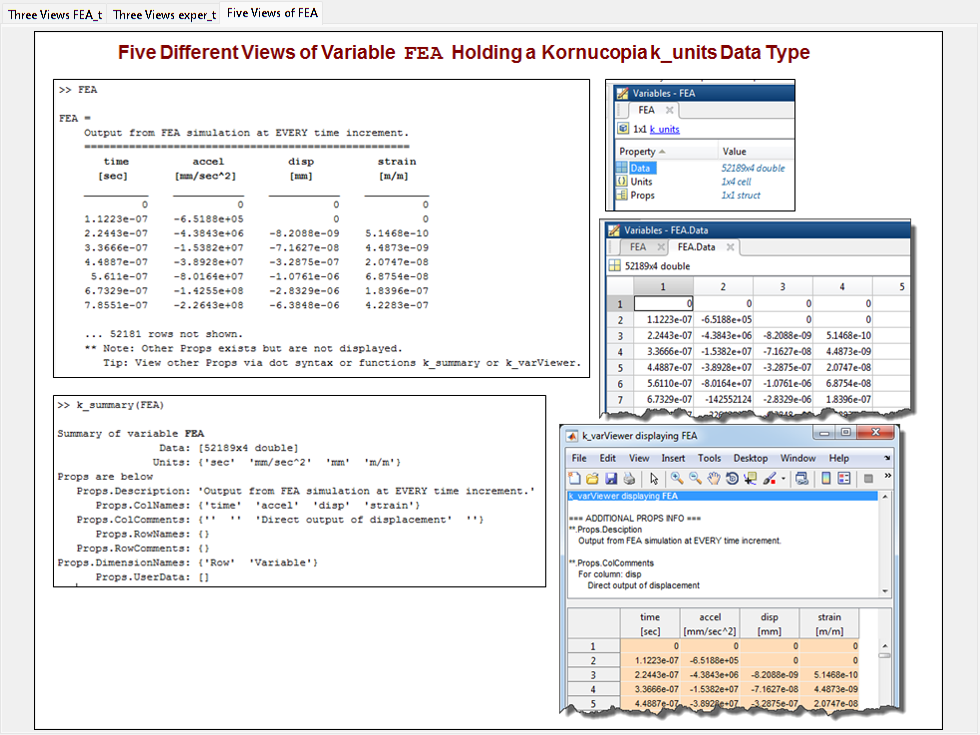
%{
Below we convert the variable FEA_t from a MATLAB table to a k_units
data type.
%}

FEA = k_units(FEA_t);

txt = {
    '*** INSTRUCTIONS FOR USER ***'
    ' '
    'AFTER you run this section, do the following: '
    ' '
    '1) Manually open the FEA variable in the MATLAB editor. '
    '     - What do you see? (It looks like a structure). '
    ' '
    '2) Next issue the following commands in the MATLAB Command Window: '
    '      display(FEA)'
    '      FEA  % This will produce result same as above'
    '      k_summary(FEA)'
    '      k_varViewer(FEA)'
    ' '
    'You should have observed some of the differences of how a MATLAB '
    'table presents the data and how a Kornucopia table (k_units data '
    'type) presents the data to the user.'
    ' '
    'Once you are done, run the next section to see pictures of '
    'what you should have experienced. '
    };

msgbox(txt, 'Instructions');
Display picture of 5 possible ways to view k_units variable in MATLAB
% Add a tab to display the picture
refTabH = tabStuff.TabsH(2);
tabStuff = k_figTabsInsert('Five Views of FEA', 'after', refTabH);
currentTabH = tabStuff.TabsH(3);

imageName = 'fiveViews_FEA.png';
fullImageName = fullfile(dataDir, 'media', imageName);
k_picDisplay(fullImageName, 'center', ...
    'parent', currentTabH);
k_figTabsDisplay(currentTabH);
Viewing the Kornucopia Units Library
%{
The next couple of commands provide different listing options to see
the various units in the Kornucopia Units Library.

You may desire to try running the interactive command a few times to
try out the various options.
%}

k_unitsList('-groups')

disp(' '), disp(' ')

k_unitsList() % Show Full List Interactively
    Group Name           Units in Group
    _________________    ______________________________________________________
    absTemperature       degK, degR, K, R, °K, °R
    acceleration         G, kG, mG
    angle                arcmin, arcsec, deg, mrad, rad, rev, urad, °
    angularFreq          cps, RPM, rpm
    area                 acre
    capacitance          F, GF, kF, MF, mF, nF, pF, uF, µF
    celsius              degC, °C
    charge               C, GC, kC, MC, mC, nC, pC, uC, µC
    conductance          GS, kS, MS, mS, nS, S, uS, µS
    currency             currency
    current              A, mA
    energy               BTU, Cal, cal, Cal_IT, cal_IT, J, kcal, kcal_IT, kJ,
                         MJ, mJ, uJ, µJ
    fahrenheit           degF, °F
    force                cN, dN, dyn, dyne, gf, gmf, kgf, kip, kN, lbf, mN, N,
                         nN, ozf, pN, uN, µN
    forcePerLength       pli
    frequency            GHz, Hz, kHz, MHz, THz
    fundamental          A, cd, currency, item, K, kg, m, mol, rad, s
    illuminance          lux, lx
    inductance           GH, H, kH, MH, mH, nH, pH, uH, µH
    item                 item
    length               cm, dm, ft, furlong, in, inch, km, m, micron, mil,
                         mile, mm, nm, um, yd, µm
    linearMassDensity    den, dtex, tex
    luminousIntensity    cd, lumen
    magnetism            fWb, Gauss, gauss, GT, GWb, kT, kWb, MT, mT, MWb, mWb,
                         nT, nWb, Oe, Oersted, oersted, pWb, T, Tesla, tesla,
                         uT, uWb, Wb, Weber, weber, µT, µWb
    mass                 blob, gm, grn, kg, lbm, Mg, mg, microgram, msnail, oz,
                         slinch, slug, snail, ton, tonne, ug, usnail, µg,
                         µsnail
    microStrain          microStrain, uStrain, µStrain
    miscellaneous        %, 1, GSa, kSa, micro, MSa, Sa, TSa, µ
    percent              %
    potential            GV, kV, microV, MV, mV, nV, pV, uV, V, µV
    power                GW, hp, kW, MW, mW, nW, uW, W, µW
    pressure             atm, bar, GPa, inHg, kPa, ksi, mbar, mmHg, MPa, Pa,
                         psf, psi, torr
    resistance           Gohm, kohm, Mohm, mohm, nohm, ohm, uohm, µohm
    strain               microStrain, milliStrain, mStrain, uStrain, µStrain
    substance            mol
    temperature          degC, degF, degK, degR, K, R, °C, °F, °K, °R
    textile              cottonCount, den, dtex, gpd, mgpd, tex
    time                 day, fortnight, hr, microsec, min, minute, ms, msec,
                         ns, nsec, s, sec, us, usec, µs, µsec
    userDefined
    velocity             fps, ips, knot, kph, mph
    viscosity            cP, Poise, poise
    volume               cc, floz, galUK, galUS, L, mL


    unit    originalFormula    baseDefShort           description    groups       source
    ____    _______________    ___________________    ___________    _________    __________
    GHz     GHz = 1e9*Hz       GHz = 1.000e+09*1/s    gigahertz      frequency    Kornucopia
    Hz      Hz = 1/s           Hz = 1.000*1/s         hertz          frequency    Kornucopia
    kHz     kHz = 1e3*Hz       kHz = 1000*1/s         kilohertz      frequency    Kornucopia
    MHz     MHz = 1e6*Hz       MHz = 1.000e+06*1/s    megahertz      frequency    Kornucopia
    THz     THz = 1e12*Hz      THz = 1.000e+12*1/s    terahertz      frequency    Kornucopia
Convert exper_t to k_units data type
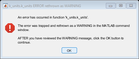
%{
Below we try to convert the MATLAB table exper_t to a k_units data
type.

The initial attempt produces an error due to a units issue. READ the
error pop-up and related message that is displayed in the MATLAB
Command Window.

Note: This following will create an error.
Please read the error message for what is wrong.
%}

try
    exper = k_units(exper_t);
catch err
    k_errToWarn(err);
end
Warning: An error has occurred in function 'k_units.k_units'.

PLEASE READ: The units string 'g' is NOT defined by default in Kornucopia
because in practice some use 'g' for gram mass while others use it for a unit of
acceleration. Below are several options you can utilize to deal with units of
'g':
   1) For gram mass use 'gm' or '0.001*kg'
   2) For acceleration use 'G'
   3) Define 'g' to be either gram mass or acceleration via:
      k_unitsDefine('g = 0.001*kg', 'gram mass', 'mass')
      OR
      k_unitsDefine('g = 9.806650*m/s^2', 'accel of gravity', 'acceleration')
Please note that options 1 and 2 above assume you have not already re-defined
'gm' or 'G'.
Click this link for <a href="matlab: zzqKorn.launchKornHelpBrowser('k_units');">detailed help on k_units</a>
Define unit of 'g' and re-attempt converting exper_t to k_units
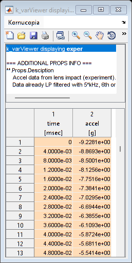
%{
It is easy to add (or delete) units from the Kornucopia Units Library.
As explained in the error message in previous section, the unit of 'g'
is not predefined in the Library, but the unit of 'G' is predefined as
1 unit of Earth's gravity.

Below we put 'g' into the library and then convert exper_t
%}

k_unitsDefine('g = G') ;
exper = k_units(exper_t);

% Below we display variable to command window and also in k_varViewer
display(exper)
k_varViewer(exper)
exper =
    Accel data from lens impact (experiment).
    Data already LP filtered with 5*kHz, 6th order, bi-directional Butter filter.
    =============================================================================
      time      accel
     [msec]      [g]
    ________    ______
       0.000    -9.228
    0.004000    -8.869
    0.008000    -8.500
     0.01200    -8.126
     0.01600    -7.752
     0.02000    -7.384
     0.02400    -7.030
     0.02800    -6.694

    ... 1693 rows not shown.
        See "n" rows via k_set('dispBrief', n).
Compare the FEA and Experimental Data
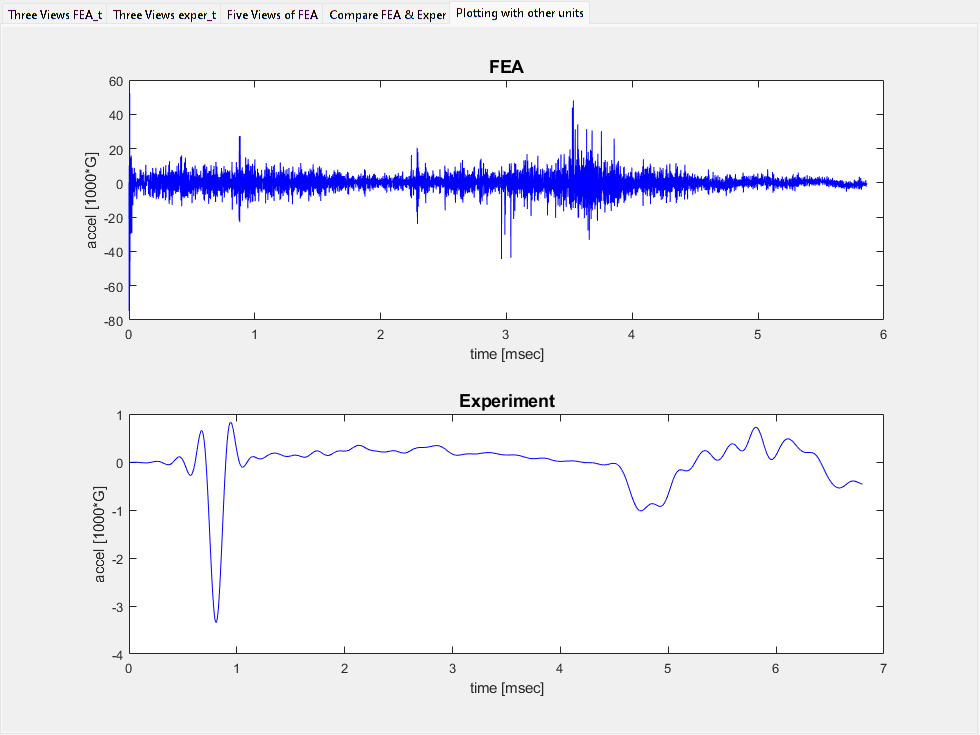
%{
Below we make a plot to compare the FEA and Experimental data.
We use the variable versions that are of k_units data type because it
will make plotting and other mathematical operations easier than
working with a MATLAB table data type.

In the plot calls below, we show using ADV option 'dependentCol' where in
the first use we spell-out the option fully, but in the 2nd case we
demonstrate a commonly used abbreviation.
%}

% Add a tab to display the picture
refTabH = tabStuff.TabsH(3);
tabStuff = k_figTabsInsert('Compare FEA & Exper', 'after', refTabH);
currentTabH = tabStuff.TabsH(4);

subplot(2,1,1, 'parent', currentTabH)
k_plot(FEA, [], ...
    'dependentCol', 'accel', ...
    'title', {'user', 'FEA'})

subplot(2,1,2)
k_plot(exper, [], ...
    'depend', 'accel', ...
    'title', {'user', 'Experiment'})

k_figTabsDisplay(currentTabH);

% Shown below is how to make a similar plot without k_plot and k_units
% variable types. It is a bit more work!
%{

figure

subplot(2,1,1);
plot(FEA_t.time, FEA_t.accel)
xlabel(['time [',FEA_t.Properties.VariableUnits{'time'}, ']']);
ylabel(['accel [', FEA_t.Properties.VariableUnits{'accel'}, ']']);
title('FEA', 'fontWeight', 'bold')

subplot(2,1,2);
plot(exper_t.time, exper_t.accel)
xlabel(['time [',exper_t.Properties.VariableUnits{'time'}, ']']);
ylabel(['accel [', exper_t.Properties.VariableUnits{'accel'}, ']']);
title('Experimental', 'fontWeight', 'bold')
%}


% Below we re-make the plots but with more reasonable units.

refTabH = tabStuff.TabsH(4);
tabStuff = k_figTabsInsert('Plotting with other units', 'after', refTabH);
currentTabH = tabStuff.TabsH(5);

subplot(2,1,1, 'parent', currentTabH)
k_plot(FEA, [], ...
    'depend', 'accel', ...
    'title', {'user', 'FEA'}, ...
    'unitsConvertTo', 'msec, 1000*G')

subplot(2,1,2)
k_plot(exper, [], ...
    'depend', 'accel', ...
    'title', {'user', 'Experiment'}, ...
    'unitsConvertTo', 'msec, 1000*G')

k_figTabsDisplay(currentTabH);
Comparing displacements by integrating accelerations
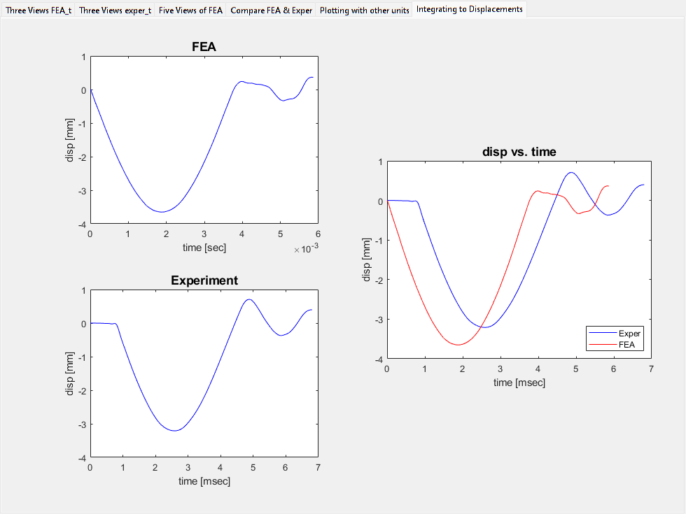
%{
In this section we demonstrate how easy it is to work with data
numerically, in this case integrating acceleration vs time to yield
velocities and then displacements.

Note in this example, there is no initial velocity so we can ignore
the third (optional) argument of the k_integrate function.

The plotting demonstrated is a bit more fancy too.
%}

% Integrate first to velocity and then to displacement
v = k_integrate(exper('time'), exper('accel'));
exper{'disp'} = k_integrate(exper('time'), v, '0*m');

% Note: using curly braces above, "exper{'disp'} =" told Kornucopia to add
% a new column to end of exper that has column name 'disp'.

% Plot the results
refTabH = tabStuff.TabsH(5);
tabStuff = k_figTabsInsert('Integrating to Displacements', 'after', refTabH);
currentTabH = tabStuff.TabsH(6);

subplot(2,2,1, 'parent', currentTabH)
k_plot(FEA, [], ...
    'depend', 'disp', ...
    'title', {'user', 'FEA'})

subplot(2,2,3)
k_plot(exper, [], ...
    'depend', 'disp', ...
    'title', {'user', 'Experiment'})

% For the combo plot below, Kornucopia knows how to automatically
% convert the data sets to common units for the plot.
aH = axes('parent', currentTabH, ...
    'OuterPosition', [0.5, 0.25, 0.5, 0.5]);

toPlot = {exper, FEA};
k_plot(toPlot, [], ...
    'parent', aH, ...
    'depend', 'disp', ...
    'legendText', {'user', {'Exper', 'FEA'}}, ...
    'legendLocation', 'SouthEast')

k_figTabsDisplay(currentTabH);
Convert the FEA and Exper variables to a common Units Pref
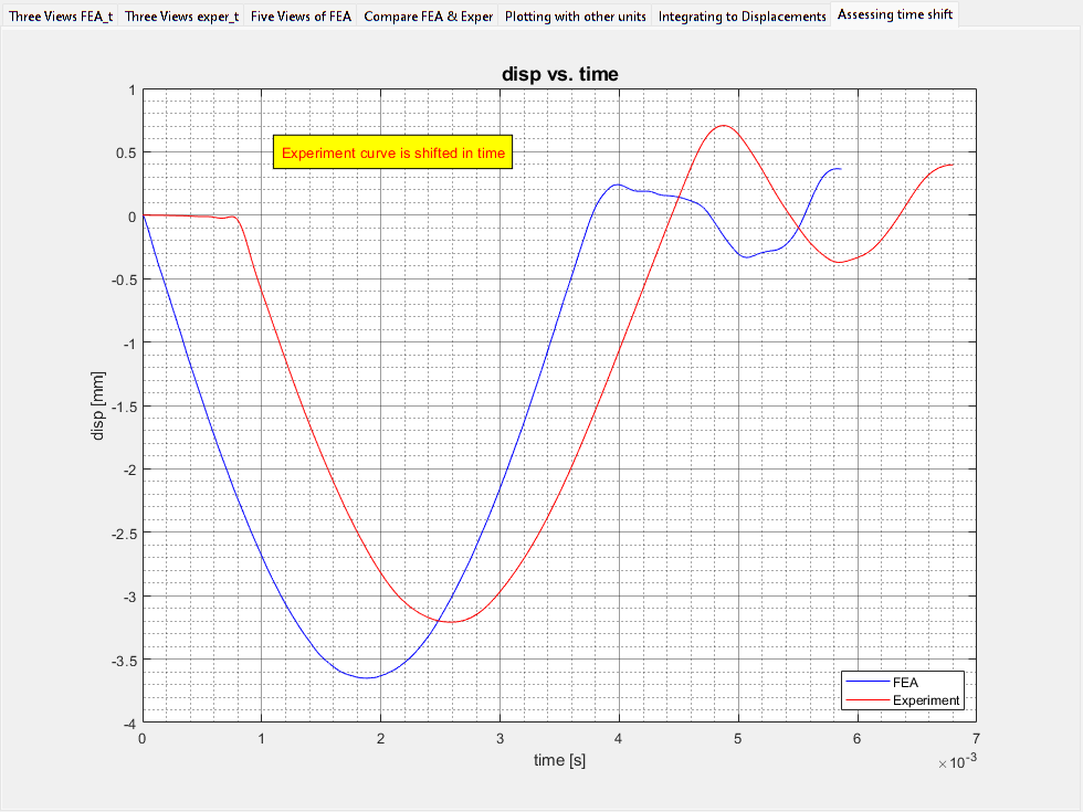
%{
Kornucopia can easily and properly handle datasets in different units.
However, many users like to see their data in a common set of units.

Below we allow you, the user, to select a units system from the pop-up
and then Kornucopia will convert the data to that set of units.
%}

% Interactively select Units Pref
k_unitsPreferenceActivate();

% Perform the conversion on each variable (all columns get converted)
FEA = FEA.convert();
exper = exper.convert();

% For simplicity, change the description to each variable, but place
% the original description in UserData property for traceability
FEA.Props.UserData.OrigDescription = FEA.Props.Description
FEA.Props.Description = 'FEA';
exper.Props.UserData.OrigDescription = exper.Props.Description
exper.Props.Description = 'Experiment';

% Make a nice plot
refTabH = tabStuff.TabsH(6);
tabStuff = k_figTabsInsert('Assessing time shift', 'after', refTabH);
currentTabH = tabStuff.TabsH(7);

toPlt = {FEA, exper};
k_plot(toPlt, [], ...
    'parent', currentTabH, ...
    'legendLocation', 'SouthEast', ...
    adv.k_plot.grid.bothMajorMinor, ...
    adv.k_plot.dependentCol, 3) % Showing flexiblity of using index

k_displayOnFigure(0.3, 0.9, 'Experiment curve is shifted in time', ...
    'box', 'on', ...
    'boxFillColor', 'yellow', ...
    'fontColor', 'red')

k_figTabsDisplay(currentTabH);
Units Preference now activated: 'mm_N_s'

FEA =
    Output from FEA simulation at EVERY time increment.
    ===================================================
      time         accel          disp        strain
       [s]        [mm/s^2]        [mm]
    _________    __________    __________    _________
        0.000         0.000         0.000        0.000
    1.122e-07    -6.519e+05         0.000        0.000
    2.244e-07    -4.384e+06    -8.209e-09    5.147e-10
    3.367e-07    -1.538e+07    -7.163e-08    4.487e-09
    4.489e-07    -3.893e+07    -3.287e-07    2.075e-08
    5.611e-07    -8.016e+07    -1.076e-06    6.875e-08
    6.733e-07    -1.426e+08    -2.833e-06    1.840e-07
    7.855e-07    -2.264e+08    -6.385e-06    4.228e-07

    ... 52181 rows not shown.
        See "n" rows via k_set('dispBrief', n).
     ** Other Props exist that are not displayed.
        View other Props via dot syntax or functions k_summary or k_varViewer.


exper =
    Accel data from lens impact (experiment).
    Data already LP filtered with 5*kHz, 6th order, bi-directional Butter filter.
    =============================================================================
      time         accel          disp
       [s]        [mm/s^2]        [mm]
    _________    __________    __________
        0.000    -9.050e+04         0.000
    4.000e-06    -8.698e+04    -7.147e-07
    8.000e-06    -8.336e+04    -2.821e-06
    1.200e-05    -7.968e+04    -6.261e-06
    1.600e-05    -7.602e+04    -1.098e-05
    2.000e-05    -7.241e+04    -1.691e-05
    2.400e-05    -6.894e+04    -2.400e-05
    2.800e-05    -6.565e+04    -3.219e-05

    ... 1693 rows not shown.
        See "n" rows via k_set('dispBrief', n).
     ** Other Props exist that are not displayed.
        View other Props via dot syntax or functions k_summary or k_varViewer.
Shift time of Experiment and replot
%{
Using the MATLAB Data Cursor, we estimate the time shift to be 0.78*ms.
Note, the Data Cursor feature does not report the values with units,
just the number from the graph.

Below we try to shift the time data but forget to include units, and
thus generate a units-related error.
Please read the message that appears.
%}
try
    exper('time') = exper('time') - 0.78;
catch err
    k_errToWarn(err)
end
Warning: An error has occurred in function 'k_units.minus'.

Incompatible units error. The following two units do not resolve to the same
primary units signature:
   's' and ''.
Click this link for <a href="matlab: zzqKorn.launchKornHelpBrowser('k_units');">detailed help on k_units</a>
Click this link for <a href="matlab: zzqKorn.launchKornHelpBrowser('Overloaded_MATLAB_functions');">details on overloaded MATLAB functions.</a>

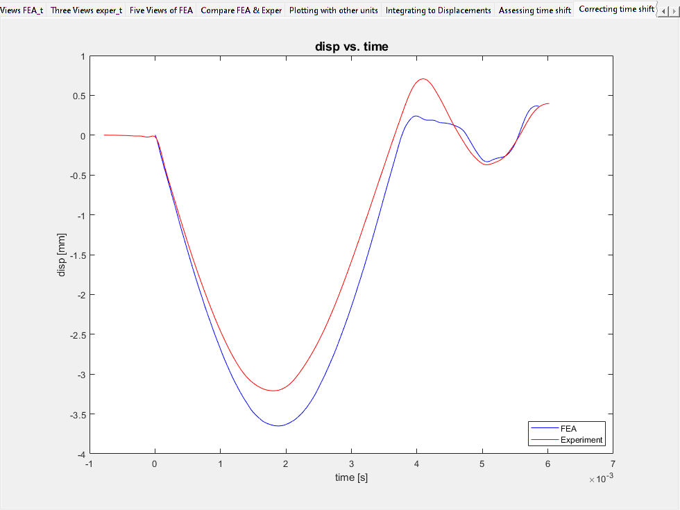
Shift time of Experiment using units and replot
%{
We need to put units with the "0.78".
Below we demonstrate the flexibility of using strings for units under
cases when a k_units variable (exper in this example) is part of a
math operation. This is leveraging Kornucopia-Compatible Data Types.

*** Caution ***
If you re-run this section multiple times, you will keep subtracting
the time shift from the data, resulting in it being shifted too much.
%}

exper_copy = exper; % used to demonstrate two ways to shift the data

% Doing subtracting using Kornucopia-Compatible Data Types
exper('time') = exper('time') - '0.78*ms';

% The more tradtional way
k_unitsVariables('ms') % This creates a variable ms which is 1*ms
exper_copy('time') = exper('time') - 0.78*ms;

% Plot the results
refTabH = tabStuff.TabsH(7);
tabStuff = k_figTabsInsert('Correcting time shift', 'after', refTabH);
currentTabH = tabStuff.TabsH(8);

toPlt = {FEA, exper};
k_plot(toPlt, [], ...
    'parent', currentTabH, ...
    'legendLocation', 'SouthEast', ...
    adv.k_plot.dependentCol, 3)

k_figTabsDisplay(currentTabH);
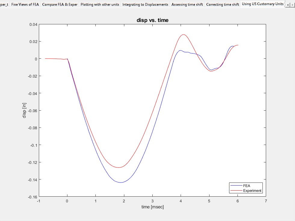
Convert to US Customary units and make time in msec, then replot
%{
This section converts the data to a form of US Customary units.
%}

% change the units preference to this system.
k_unitsPreferenceActivate('in_lbf_slinch_s')

% Convert the variables and then make extra conversion from s to msec
FEA = FEA.convert();
FEA('time') = FEA('time').convert('msec');
exper = exper.convert();
exper('time') = exper('time').convert('msec');

% Plot the results
refTabH = tabStuff.TabsH(8);
tabStuff = k_figTabsInsert('Using US Customary Units', 'after', refTabH);
currentTabH = tabStuff.TabsH(9);

toPlt = {FEA, exper};
k_plot(toPlt, [], ...
    'parent', currentTabH, ...
    'legendLocation', 'SouthEast', ...
    adv.k_plot.dependentCol, 3)

k_figTabsDisplay(currentTabH);
Units Preference now activated: 'in_lbf_slinch_s'
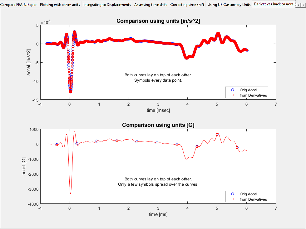
Demonstration of computing a derivative
%{
This last section demonstrates computing two successive derivatives of
the experimental displacement to obtain acceleration and then compare
that result to the original acceleration.
%}

vExper = k_derivative(exper('time'), exper('disp'));
aExper = k_derivative(exper('time'), vExper);
aExper.Props.ColNames = 'accel';

% Plotting the results
refTabH = tabStuff.TabsH(9);
tabStuff = k_figTabsInsert('Derivatives back to accel', 'after', refTabH);
currentTabH = tabStuff.TabsH(10);

% The first plot has accel units of in/s^2
subplot(2,1,1, 'parent', currentTabH)
titleTxt = ['Comparison using units [', exper.Units{'accel'}, ']'];

k_plot(exper('time'), {exper('accel'), aExper}, ...
    'markerSymbols', 'list', ...
    'legendText', {'user', {'Orig Accel', 'from Derivatives'}}, ...
    'legendLocation', 'best', ...
    'title', {'user', titleTxt})

msgTxt = {'Both curves lay on top of each other.';...
          'Symbols every data point.'};
k_displayOnFigure(0.5,0.3, msgTxt);


% Using the ADV option unitsConvertTo we can easily change the units
% of the plot without changing the units of the variables directly.
% Also controlling the number of symbol markers.
subplot(2,1,2)
titleTxt = 'Comparison using units [G]';

k_plot(exper('time'), {exper('accel'), aExper}, ...
    'markerSymbols', 'list', ...
    'markerOccurrence', {'total', 10}, ...
    'legendText', {'user', {'Orig Accel', 'from Derivatives'}}, ...
    'legendLocation', 'best', ...
    'unitsConvertTo', 'ms, G', ...
    'title', {'user', titleTxt})

msgTxt = {'Both curves lay on top of each other.';...
          'Only a few symbols spread over the curves.'};
k_displayOnFigure(0.5,0.3, msgTxt);

k_figTabsDisplay(currentTabH);
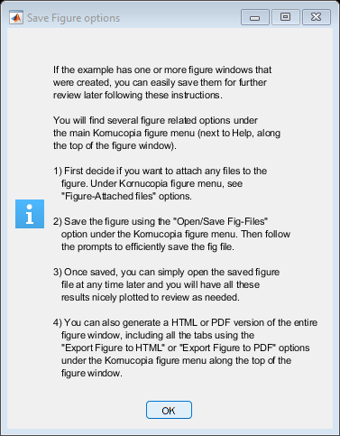
Options to save figure windows
k_exampleSetup('figSavingOptions');
End of example & optional clean-up
%{
Additional Details:
This section does the following:
 o Offer the user the option to delete the 'g' units definition
   created earlier.
 o Resets any changed preferences, such as Units Preferences and
   default ADV values back to their state prior to the example.
 o Resets the MATLAB format setting back to its original state prior
   to the example.
 o Opens an interactive dialog to offer the option of cleaning-up the
   MATLAB workspace.
%}

msgTxt = {['Note: The unit ''g'' was defined and added to the ', ...
    'Kornucopia Units Library during this example. '], ' ', ...
    'Do you want it deleted from the MATLAB session? '};
q = questdlg(msgTxt);

if strcmpi(q, 'Yes')
    try
        k_unitsDefine('g = []');
    catch
    end
end

k_exampleSetup(origSettings);
Units Preference now activated: 'ShockVib_mm_ms_G'